
Calculated variables
Presentation of calculated variables
In the tab "Variable" one can identify easily the variables which one would like to receive in Data Hub. The variables (raw variables) that are received via a third system (hardware or other source) and the virtual variables (“calculated” variables) that are calculated via a combination a specific variable of the specific source with other data sources available in Data Hub. Please, make sure to read our "Best Practices" section before defining any calculated variable.
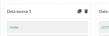
One can easily distinguish the raw variables from the virtual variables via a symbol indicated in the image here-under.
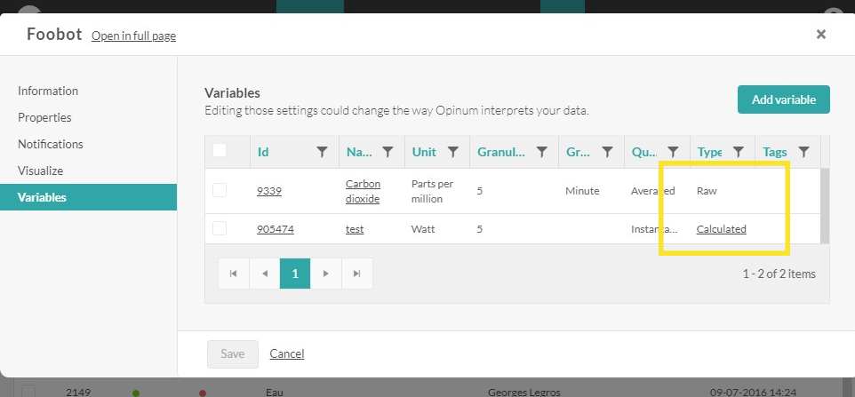
E.g. in this case the variable "Phase A consumption" is a variable indicating a consumption based on the raw variable received: "Phase A Index".
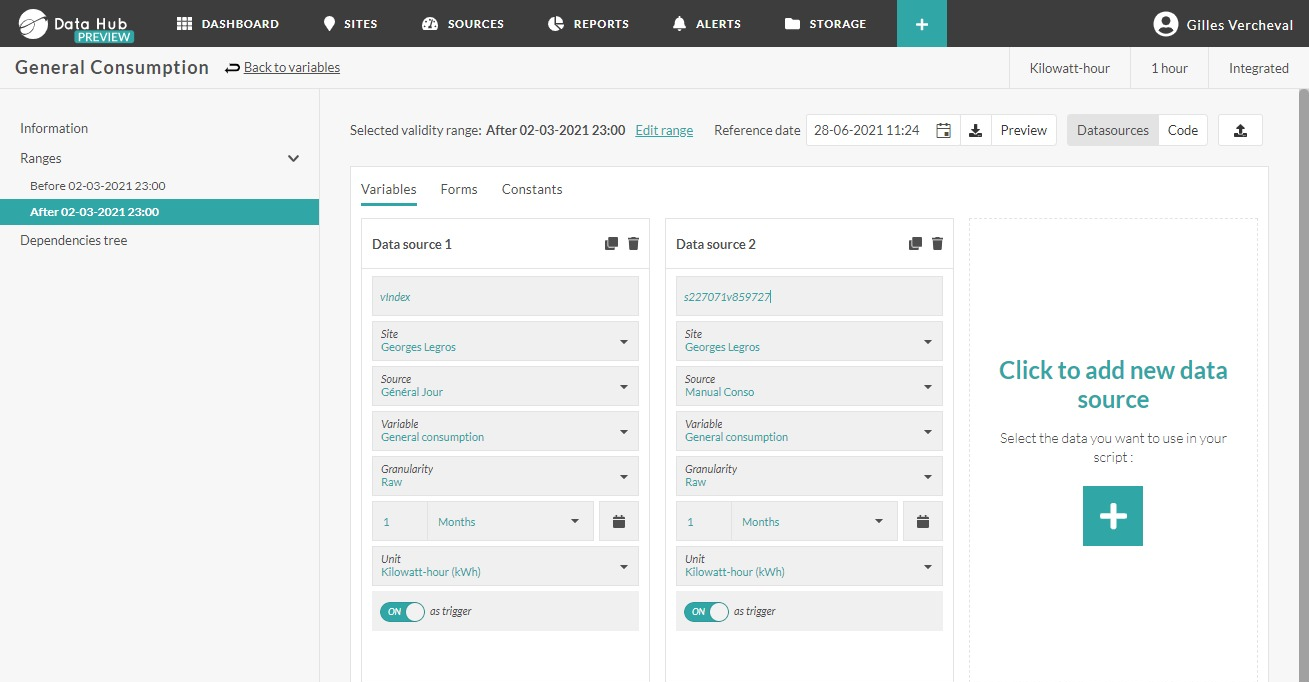
The interface for configuration is split in two parts:
At the left: one can see a configuration tool and select variables that will be combined via the calculation. In this case, one has indicated the sources which will be used to calculate a virtual variable. Apart from variables related to sources that are available in Opinum, one can also define a constant value via the tab Forms.
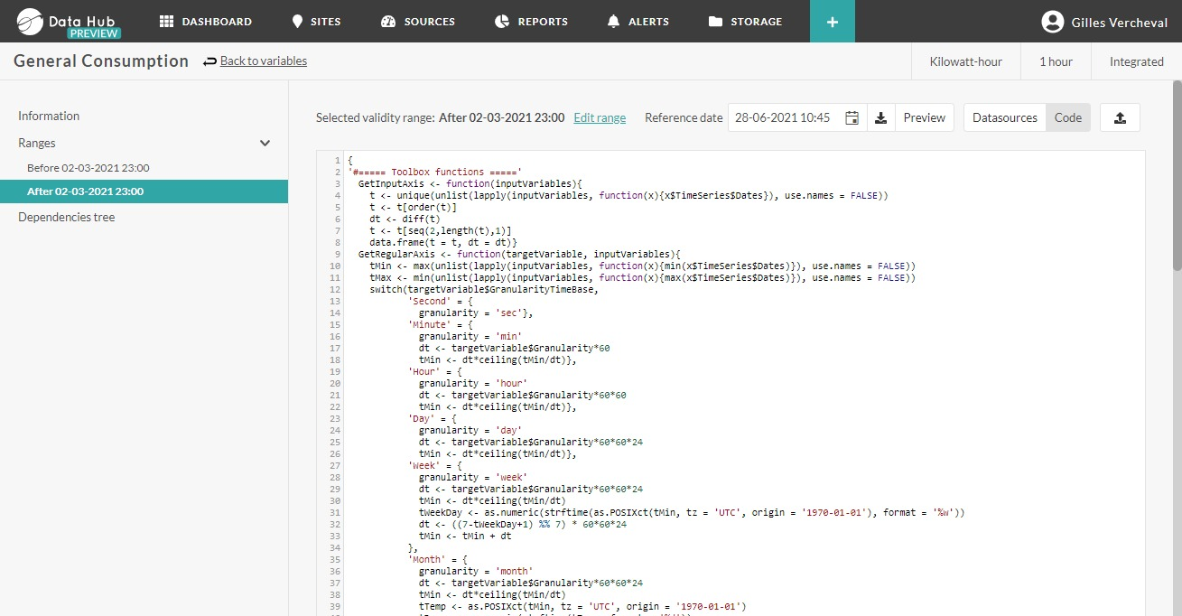
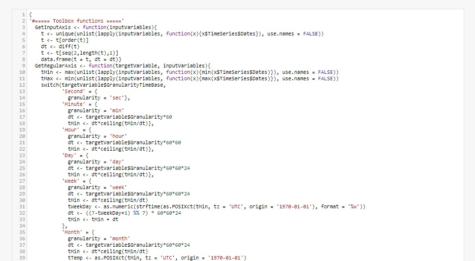
At the right: the code permits to calculate the virtual variable based on the variables that are selected. In this case, the user uses a code in language R.
The code that is used by the client is a standard code in Opinum. This code is a code to calculate the consumption based on index values.
The engine of the operation is stipulated in the section “Formula”:

We see that the result of the virtual variable will be calculated based on the successive difference of the index values.
The rest of the code is used for:
- Separate the different variables on an time axis (t$t), which will be used for the calculated variable (functions GetInputAxis, GetRegularAxis, SetDataOnCommonAxis)
- Filter the result of the calculated variables in order to ignore the points that are exactly the same as those that are already present in Opinum (functions FilterNaOutput et FilterDuplicateOutput)
For more detailed explication on the functions and on the working method of the calculated variables, follow the link to the Webinar on the calculated variables:.
Here-under we provide some important notes in relation with the way to access the input variables.
If ‘x’ is the alias which is given to a input variable via the interface on the left:
- -inputVariables$x$TimeSeries$Dates permits to access the time axis from the input variable
- -inputVariables$x$TimeSeries$Values permits to access the values of the input variable
- -inputVariables$x$TimeSeries permits to access the table with two vectors referred to: at each time stamp, the value
In order to receive more insights on all the functionalities of the interface “Calculated variables”, image that we will calculate the consumption of a value starting from an index value:
Creation and use of calculated variables
Introduction
Imagine that we will calculate a virtual variable for consumption (which we call “Total consumption”) from an index value (which is called “Active energy” in this example. In order to start, one will click on "Add a new calculated variable" in the tab Config.
The following screen asks us to define a new calculated variable.
- Type of calculation: At this point, only language R is supported. The implementation of other languages is foreseen.
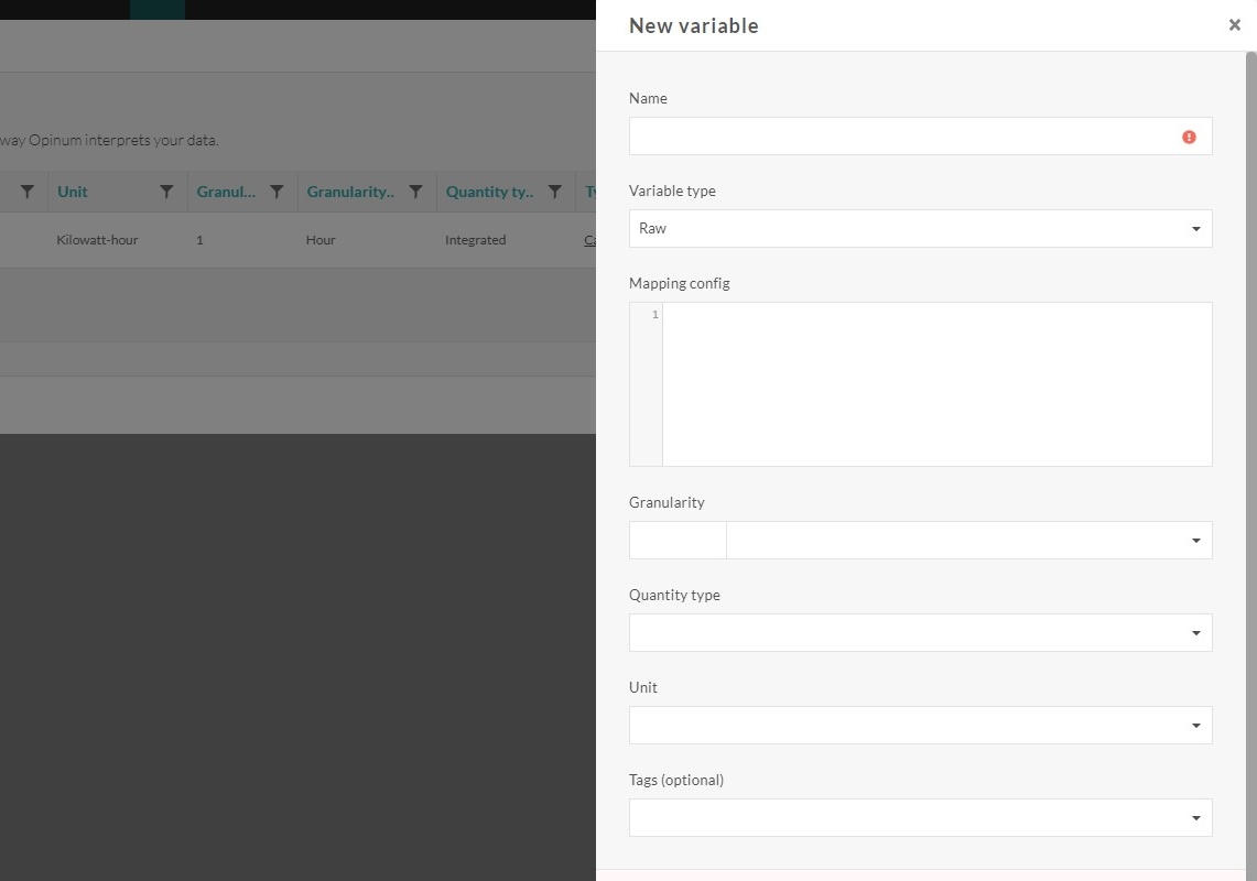
- Name: Name of the new calculated variable
- Unit: unit of the values of the calculated variables (when the calculation is performed). One should think about the grandeur of the results of the calculated variables so that the unit chosen is in line with the calculation.
- Granularity: the granularity of the variable indicates the time between each value of the calculated variable (e.g. hourly, daily).
- Quantity type:
- Instantaneous: characterizes an instantaneous variable which has a specific value at a moment in time (typical: stream, frequency, voltage, power, debit ...)
- Integrated: characterizes a variable from which the grandeur ensues from an integration (typical: energy consumption)
- Cumulative : characterizes a variable which will only accumulate (typical: a consumption index).
- Minimum: characterizes a variables from which the value will be the minimum value in a time interval (typical: minimum stream, minimum frequency, minimum voltage, minimum power, minimum debit, ...)
- Maximum: characterizes a variable from which the value will be the maximum value in a time interval (typical : maximum stream, maximum frequency, maximum voltage, maximum power, maximum debit, ... )
- Averaged: characterizes a variable from which the value will be the average value in a time interval (typical : average stream, average frequency, average voltage, average power, average debit, ... )
- When clicking on “Save”, the interface will switch immediately to the interface for the real configuration of the virtual variable:
Definition of the variables to include
A first step consists out of the definition to define the variables to include in the calculation.
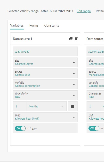
- Alias: name which will be given to the input variable in the calculation. This alias is used in the syntax: inputVariables$x$TimeSeries.
- Site: site to which the input variable is linked
- Source: source to which the input variable is linked
- Variable : input variable
- Granularity: by choosing "Raw", one chooses not to aggregate the values from the input variables. By choosing not for the option “Raw”, the input data will be aggregated based on your choice: minute, hour, day, week, month or year, before sending over the data to the calculation engine. ,
- Aggregation: if the granularity is not "Raw", one should choose the method of aggregation: sum, average, maximum, when appearing, variance or standard deviation.
- Period: the period permits to define the quantity of data input which will be send over to the calculation engine, at each new calculation. This period can be defined by using a relative manner (2 days before, the 10 latest measuring points,…) or by using a fixed manner by choosing dates via a calendar.
- Unit: the values of the input variable will be converted in the unit chosen, before sending the values to the calculation engine.
- As trigger: by activating these fields, one will assure that a new calculation will be performed each time a new value of the chosen input variable enters Opinum. Opinum recommends to always have this option activated for at least one variable, in order to ensure that the calculation engine is activated and the virtual variable will be calculated.
Following the same logic, one can use the forms or define a constant variable as input value. In order to do this, one has to define an alias and will select a from or define a value for the constant. The two icons permit to delete an input variable or to duplicate the values of the fields in another input variable.
Implement the calculation code
The second part consists out of the implementation of the code R which will feed the calculation engine.
The output of the code should have the following form: list(Timeseries = data.frame(Dates = myDates, Values = myValues))
In this case, we can easily copy the code we used before as we used the same alias for the index variable (which is the only input value in this case), 'vIndex', we can copy the code completely in order to realise the calculation and so to have a value for the consumption. Please note that the calculation code will send back the values which are not coherent with the units which are chosen for the calculated variable (at step 1 Introduction).
Verification tool

The button "Check" permits to verify the syntax of your code in R.
The button “Visualize” permits to visualize the result via a graph showing the result of your code, based on the calculation.
If you observe a behavior which is not in line with your expectations, two possible intermediate solution can help to define the problem:
Once you defined all your input variables, you can click on "Download sample data" in order to download the data set you defined. This data set will be used in the R environment, as for example RStudio. This data set will be send to the calculation engine at each trigger (as defined). The aggregation parameters, the period and the conversion unit are already applicable on this particular data set.
You can as well make a direct export of you R code by clicking on “Add”. Your code will be directly be exploited in an R environment, like for example RStudio.
These two mechanisms permit to turn your calculation in an R environment with as goal, for example, to use a debug tool.
Best practices
This section provides a detailed explanation of how to configure calculations within Data Hub, particularly regarding the triggering of calculations and the management of associated time-series data. We will also cover best practices to ensure optimal configuration that preserves system performance while ensuring the longevity of calculations.
Triggering Calculations
Calculations are automatically triggered for every data point entering the source variables of the calculation. For a calculation to be triggered, the source variable must be marked as a "trigger."
Tip
Ensure that only essential variables are marked as "triggers" to avoid unnecessary calculations, which could affect system performance.
Managing Historical Data
When a calculation is triggered, it includes all historical data (in terms of date and time) up to the injected point. These data are limited to the period defined for each data source.
Tip
Proper configuration of the period is crucial to avoid processing excessive amounts of data, which could slow down the calculation or consume exces-sive resources.
Managing Future Data
In addition to historical data, the calculation also includes all future data (in terms of date and time) up to the injected point, with a maximum limit of 2 years.
Tip
The 2-year limit is a strict constraint, and it is recommended to ensure that the data needed for the calculation is included within this time window.
Cascading Calculations
When calculated variables are based on other calculated variables, calculations are triggered every time a new point is generated in the source calculated variable.
Tip
It is important to monitor cascading calculations to avoid unwanted calcula-tion loops or system overloads.
Defining the Calculation Period
The period for which a calculation is performed can be defined according to several criteria: • Minutes • Hours • Days • Weeks • Months • Years • Number of previous points
Tip
A period that is too short may overload the system due to overly frequent cal-culations. Conversely, a period that is too long may result in missing critical points. It is essential to find a balance.
Advanced Configurations: Date Ranges and Different Calculations
It is possible to define different date ranges for the same calculated variable and associate different calculations depending on the period or a specific pivot date.
Tip
Complex configurations of date ranges and calculations can become difficult to manage. Carefully document each configuration to avoid errors or unex-pected behavior.
Conclusion
This documentation aims to provide a comprehensive guide for configuring calculations in Data Hub Opinum. By following these guidelines and paying attention to the identified key points, you can ensure effective management of calculations while maintaining system performance and stability.
Key Takeaways:
- Limit the number of "trigger" variables to optimize performance.
- Carefully configure periods for historical and future data.
- Monitor cascading calculations to avoid infinite loops.
- Document complex configurations for easy maintenance.
Calculated Variable Engine Management
This section describes how to manage calculated variable engines in Data Hub Opinum. Calculated variable engines are responsible for executing the calculations defined for calculated variables.
Manager
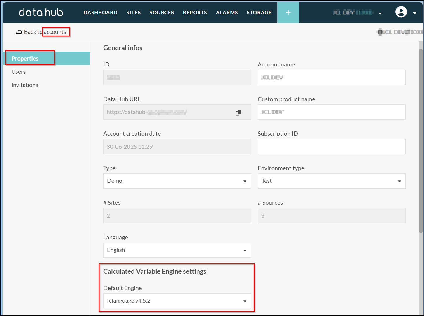
As manager, you have the ability to define default engines for new calculated variables or alter existing calculated variables to use a different engine :
Default engine: Go to properties of account and choose default engine for new calculated variables:
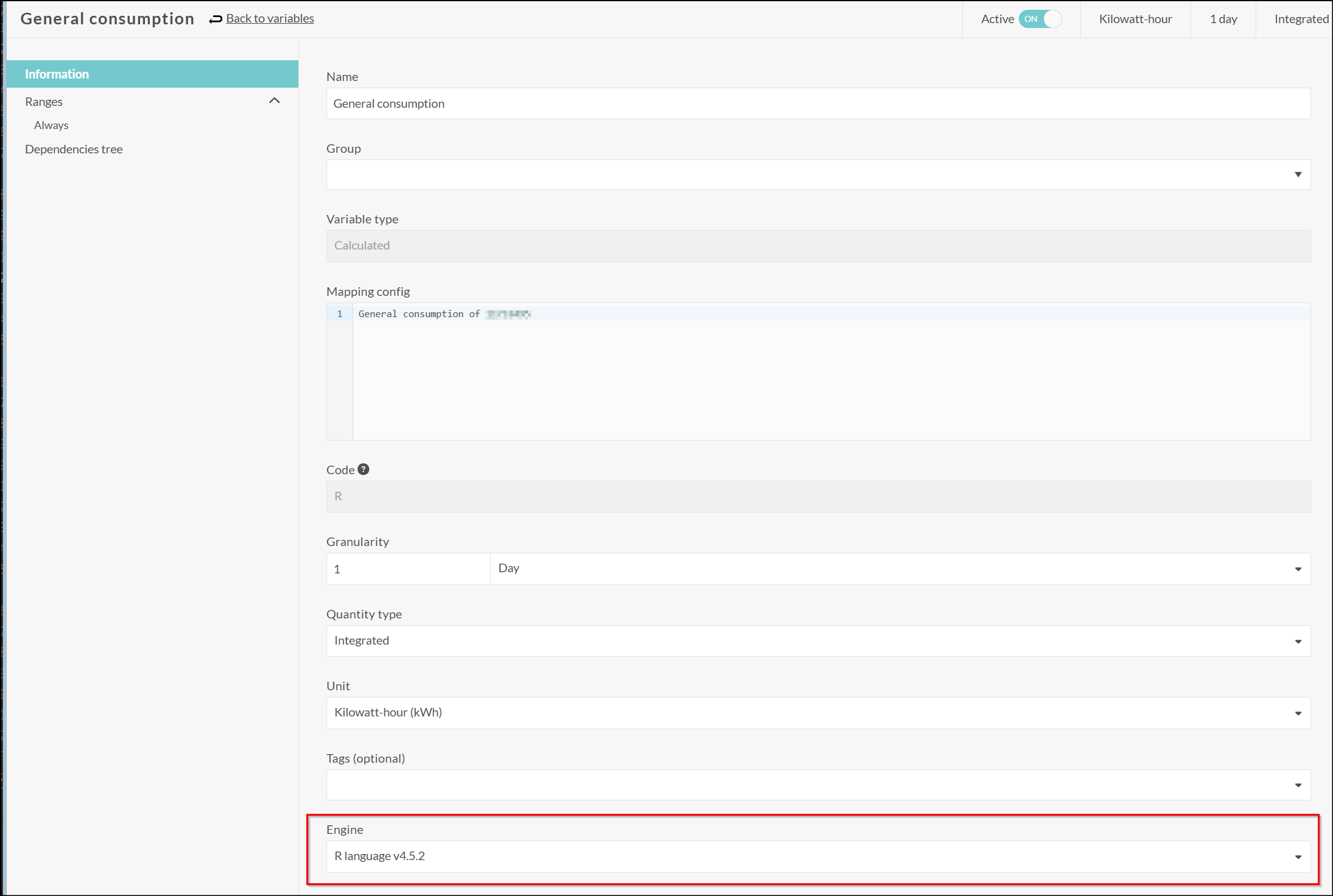
Specific: Go to information section of a calculated variable and choose engine for this variable:
Tip
Note: for more information about calculated variable engines hosted by Opinum, please contact your Opinum representative.
Administrator
As administrator, you can configure new engines for calculated variables via the Admin interface.
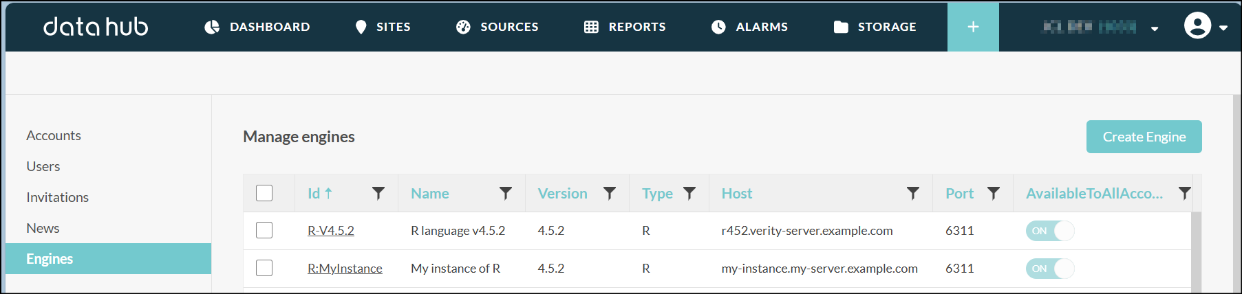
Go to admin > engines to have a list of calculated variable engines. You can add a new engine by clicking on "Create engine" button.
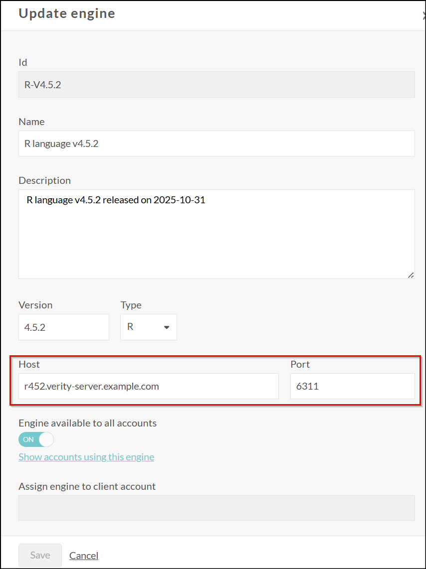
You can configure another R server on your infrastructure to be used as calculated variable engine by Data Hub Opinum. So you can choose the best infrastructure for your needs.
Then fill in the form with the information of your R server:
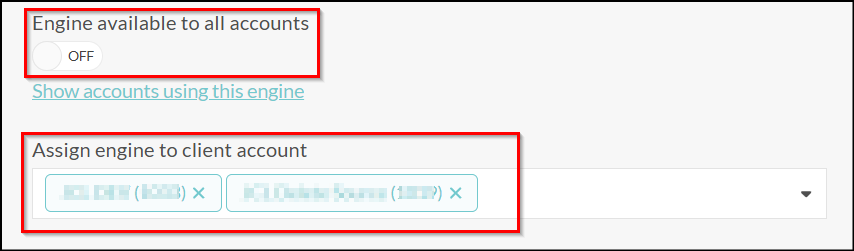
You can also configure the availability of the engine for specific accounts or for all accounts:
Tip
Note: at this time, only R engines are supported.
Installed packages on Opinum R Server
For information, here is the list of the packages installed on the Opinum R Server:
- RUN R -e "install.packages('Rserve', repos='http://cran.r-project.org')"
- RUN R -e "install.packages('ggplot2', repos='http://cran.r-project.org')"
- RUN R -e "install.packages('RJSONIO', repos='http://cran.r-project.org')"
- RUN R -e "install.packages('rjson', repos='http://cran.r-project.org')"
- RUN R -e "install.packages('Rmisc', repos='http://cran.r-project.org')"
- RUN R -e "install.packages('signal', repos='http://cran.r-project.org')"
- RUN R -e "install.packages('foreach', repos='http://cran.r-project.org')"
- RUN R -e "install.packages('doParallel', repos='http://cran.r-project.org')"
- RUN R -e "install.packages('jsonlite', repos='http://cran.r-project.org')"
- RUN R -e "install.packages('httr', repos='http://cran.r-project.org')"
- RUN R -e "install.packages('chron', repos='http://cran.r-project.org')"
- RUN R -e "install.packages('data.table', repos='http://cran.r-project.org')"
- RUN R -e "install.packages('quantmod', repos='http://cran.r-project.org')"
- RUN R -e "install.packages('oce', repos='http://cran.r-project.org')"
- RUN R -e "install.packages('RODBC', repos='http://cran.r-project.org')"
- RUN R -e "install.packages('base64enc', repos='http://cran.r-project.org')"
- RUN R -e "install.packages('lubridate', repos='http://cran.r-project.org')"
- RUN R -e "install.packages('dplyr', repos='http://cran.r-project.org')"
- RUN R -e "install.packages('forecast', repos='http://cran.r-project.org')"